Project Idea:

Generating and simulating arbitrary filters from some code. Project idea was given for the technical stage of my JITX interview for the Application Engineering position.

Problem Statement

Passive Filter Design Project

This project is meant to be a collaboration, leading you through your thought process and ability to navigate this project. Our goal with this exercise is to define, architect and implement a design generator for a large number of passive filters realizable on a user’s PCB. The filter(s) can be instantiated into user code via a function call similar to voltage-divider. The filter is instantiated as a jitx module with a fixed input/output nomenclature and using parts lookup. This is language agnostic, please choose any language of choice!

Filter Types

For this exercise, we would like eventually support of the following filter options:

RC filters
Nth order
Low pass, band pass, high pass
Spice sim verification
LC filters
Order from 1 to 7
Low pass, band pass, high pass
Bessel, Butterworth, Chebyshev, Elliptic etc
Global options
Frequency specs
Realizable components (availability)
Optimize for area or cost
Allow user to input preferences for component values
Allow user to indicate BOM consolidation priority
Initial Starting Point
To begin the exercise, we can try the following:
Start with just RC filters
LPF filter type
Three stage filter
Circuit diagram
Frequency response to component values calculation
How should we incorporate circuit and board-level non-idealities (parasitics)? Collateral Website with a nice calculator: https://rf-tools.com/lc-filter/

Basic RC Filter

  
from lcapy import *

netlist = """
R1 V_{i+} 2; right
C1 2 3; down
W 3 3; down=0, ground
W V_{i-} 3; right
W 2 V_{o+}; right
W 3 V_{o-}; right
"""
print(netlist)
cct = Circuit(netlist)

cct.draw('1st_order_rc.png', color='white')

The resulting transfer function from $V_{i}$ to $V_{o+}$

  
tf = cct.Voc('V_{i+}',  'V_{o+}').laplace()

\[\frac{1}{s + \frac{1}{C_{1} R_{1}}}\]

And we can substitute values for the capacitor and resistor with the following:

  
tf = tf.subs({
        'C1': 4,
        'R1': 5,
        })

tf.ZPK()

\[1 \cdot \frac{1}{s + \frac{1}{20}}\]

The resulting bode plot looks like.

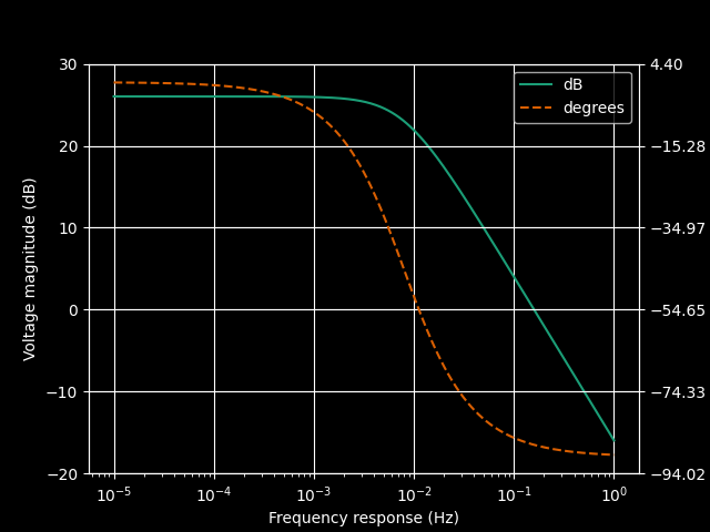
We can clearly see that the $-3dB$ point is at the pole $0.05$

But you see all the analysis above was completely wrong. Since the transfer function obtained is completely wrong as we can see from the bode plot. The response has gain greater than unity which is an obvious red flag.

The response should look like:

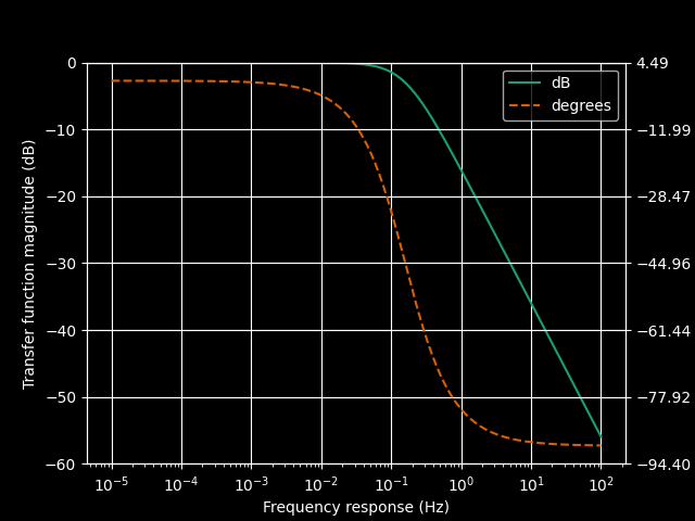
The transfer function looks like:

\[\frac{\frac{1}{C_{0}} \cdot \frac{1}{R_{0}}}{s + \frac{1}{C_{0} R_{0}}}\]

And substituting 1 for all values results in:

\[1 \cdot \frac{1}{s + 1}\]

However since we want to be able to generate a filter for some particular frequency, we must ensure that the poles are placed at the particular frequency.

To do this we can take the original transfer function and pull out the poles and solve for values that satisfy the target frequency.

Since the pole of an RC LPF filter is given by $\frac{\frac{1}{C_{0}} \cdot \frac{1}{R_{0}}}{s + \frac{1}{C_{0} R_{0}}}$ Then the pole is given by: $s + \frac{1}{C_{0} R_{0}} = 0$

\[j\omega = -\frac{1}{C_{0} R_{0}}\]

And we can now select for some values of the capacitor and resistor based on the target frequency $\omega = 2 \pi f$. Thus, we can use trial and error to solve for the closest values of R and C that match that for the frequency.

The code for that would look something like:

  
# This code finds the closest value to a given in a sorted list using a binary search

from bisect import bisect_left

def take_closest(myList, myNumber):
    """
    Assumes myList is sorted. Returns closest value to myNumber.

    If two numbers are equally close, return the smallest number.
    """
    pos = bisect_left(myList, myNumber)
    if pos == 0:
        return myList[0]
    if pos == len(myList):
        return myList[-1]
    before = myList[pos - 1]
    after = myList[pos]
    if after - myNumber < myNumber - before:
        return after
    else:
        return before

What some arbitrary cost functions might look like. They would take in a part and return the respective values.

  
def cost(x):
    return 0.5

def area(x):
    return 0.9

The actual code for identifying some the best values for a realized filter.

  
realized_filter = pd.DataFrame(columns=['RealizedFreqs', 'RealizedCaps', 'RealizedResists', 'RealizedCost', 'RealizedArea'])

for i, c in enumerate(CAPACITORS):
    r = take_closest(RESISTORS, 1/(2 * np.pi * FREQ * c))
    new_freq = 1/(2 * np.pi * r * c)

    real_cost = cost(c) + cost(r)
    real_area = area(c) + area(r)
    realized_filter.loc[i] = [new_freq, c, r, real_cost, real_area]

realized_filter_sorted = realized_filter.sort_values(by='RealizedFreqs', key=lambda x: abs(x - FREQ) )
realized_filter_sorted

With the resulting output for the realized filter looking something like the following.

	RealizedFreqs	RealizedCaps	RealizedResists	RealizedCost	RealizedArea
71	0.198864	8.200000e-06	97600.0	1.0	1.8
65	0.239807	6.800000e-06	97600.0	1.0	1.8
59	0.291194	5.600000e-06	97600.0	1.0	1.8
53	0.346954	4.700000e-06	97600.0	1.0	1.8
47	0.418125	3.900000e-06	97600.0	1.0	1.8
..	…	…	…	…	…
24	74122.086015	2.200000e-11	97600.0	1.0	1.8
18	90593.660685	1.800000e-11	97600.0	1.0	1.8
12	108712.392822	1.500000e-11	97600.0	1.0	1.8
6	135890.491028	1.200000e-11	97600.0	1.0	1.8
0	163068.589233	1.000000e-11	97600.0	1.0	1.8

Nth Order RC Filter

  
netlist = """
W 0 V_{i-}; right=0.4
"""
cct = Circuit(netlist)
# cct.add('V V_{i+} V_{i-} step 1; down')
cct.add('P1 V_{i+} V_{i-}; down, v_=v_i(t)')
for stage in range(N_STAGES):
    ground_end_node = f'G_{stage}'
    if stage == 0:
        ground_start_node = 'V_{i-}'
        start_node = 'V_{i+}'
        next_node = stage + 1
    else:
        ground_start_node = f'G_{stage-1}'
        start_node = stage
        next_node = stage + 1

    cct.add(f'R_{stage} {start_node} {next_node}; right')
    cct.add(f'C_{stage} {next_node} {ground_end_node}; down')
    cct.add(f'W {ground_start_node} {ground_end_node}; right')

vop = 'V_{o+}'
vom = 'V_{o-}'
cct.add(f'W {next_node} {vop}; right')
cct.add(f'W {ground_end_node} {vom}; right')
cct.add(f'P2 {vop} {vom}; down, v^=v_o(t)')

print()
print('Finalized netlist')
print(cct.netlist())

cct.draw(label_nodes='all', color='white')
cct.draw('3rd_order_rc_new.png', color='white')

For a 3 stage filter, that looks like:

Finalized netlist
W 0 V_{i-}; right=0.4
P1 V_{i+} V_{i-}; down, v_=v_i(t)
R_0 V_{i+} 1; right
C_0 1 G_0; down
W V_{i-} G_0; right
R_1 1 2; right
C_1 2 G_1; down
W G_0 G_1; right
R_2 2 3; right
C_2 3 G_2; down
W G_1 G_2; right
W 3 V_{o+}; right
W G_2 V_{o-}; right
P2 V_{o+} V_{o-}; down, v^=v_o(t)

The transfer function.

\[\frac{\frac{1}{C_{0}} \cdot \frac{1}{C_{1}} \cdot \frac{1}{C_{2}} \cdot \frac{1}{R_{0}} \cdot \frac{1}{R_{1}} \cdot \frac{1}{R_{2}}}{s^{3} + \frac{s^{2} \left(C_{0} C_{1} R_{0} R_{1} + C_{0} C_{2} R_{0} R_{1} + C_{0} C_{2} R_{0} R_{2} + C_{1} C_{2} R_{0} R_{2} + C_{1} C_{2} R_{1} R_{2}\right)}{C_{0} C_{1} C_{2} R_{0} R_{1} R_{2}} + \frac{s \left(C_{0} R_{0} + C_{1} R_{0} + C_{1} R_{1} + C_{2} R_{0} + C_{2} R_{1} + C_{2} R_{2}\right)}{C_{0} C_{1} C_{2} R_{0} R_{1} R_{2}} + \frac{1}{C_{0} C_{1} C_{2} R_{0} R_{1} R_{2}}}\]

  
# Sub all resistor and capacitor values for 1
Hs = tf.subs({f'C_{i}' : 1 for i in range(N_STAGES)}).subs({f'R_{i}' : 1 for i in range(N_STAGES)}).ZPK()
Hs.latex()

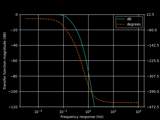
\[1 \cdot \frac{1}{s + \frac{5}{3} + \frac{7}{3 \sqrt[3]{\frac{7}{2} + \frac{21 \sqrt{3} \mathrm{j}}{2}}} + \frac{\sqrt[3]{\frac{7}{2} + \frac{21 \sqrt{3} \mathrm{j}}{2}}}{3}} \cdot \frac{1}{s + \frac{5}{3} + \frac{7}{3 \left(- \frac{1}{2} + \frac{\sqrt{3} \mathrm{j}}{2}\right) \sqrt[3]{\frac{7}{2} + \frac{21 \sqrt{3} \mathrm{j}}{2}}} + \frac{\left(- \frac{1}{2} + \frac{\sqrt{3} \mathrm{j}}{2}\right) \sqrt[3]{\frac{7}{2} + \frac{21 \sqrt{3} \mathrm{j}}{2}}}{3}} \cdot \frac{1}{s + \frac{5}{3} + \frac{\left(- \frac{1}{2} - \frac{\sqrt{3} \mathrm{j}}{2}\right) \sqrt[3]{\frac{7}{2} + \frac{21 \sqrt{3} \mathrm{j}}{2}}}{3} + \frac{7}{3 \left(- \frac{1}{2} - \frac{\sqrt{3} \mathrm{j}}{2}\right) \sqrt[3]{\frac{7}{2} + \frac{21 \sqrt{3} \mathrm{j}}{2}}}}\]

After doing the appropriate analysis and simulation, we can discover that the bode plot of the filter looks like the following.

Addendum - Standard Resistor and Capacitor values

I didn’t know this before doing this project, but there is essentially a list of standard resistor and capacitor values. They look like the following:

  
# Resistors available at 1% values
RESISTOR_ORDERS = [10**i for i in range(4)]
RESISTORS = [10.0, 10.2, 10.5, 10.7, 11.0, 11.3, 11.5, 11.8, 12.1, 12.4, 12.7, 13.0, 13.3, 13.7, 14.0, 14.3, 14.7, 15.0, 15.4, 15.8, 16.2, 16.5, 16.9, 17.4, 17.8, 18.2, 18.7, 19.1, 19.6, 20.0, 20.5, 21.0, 21.5, 22.1, 22.6, 23.2, 23.7, 24.3, 24.9, 25.5, 26.1, 26.7, 27.4, 28.0, 28.7, 29.4, 30.1, 30.9, 31.6, 32.4, 33.2, 34.0, 34.8, 35.7, 36.5, 37.4, 38.3, 39.2, 40.2, 41.2, 42.2, 43.2, 44.2, 45.3, 46.4, 47.5, 48.7, 49.9, 51.1, 52.3, 53.6, 54.9, 56.2, 57.6, 59.0, 60.4, 61.9, 63.4, 64.9, 66.5, 68.1, 69.8, 71.5, 73.2, 75.0, 76.8, 78.7, 80.6, 82.5, 84.5, 86.6, 88.7, 90.9, 93.1, 95.3, 97.6]
RESISTORS = np.outer(RESISTORS, RESISTOR_ORDERS).flatten()

# Capacitor avilable at 10% values
CAPACITOR_ORDERS = [10**i for i in range(-12, -6)]
CAPACITORS = [10, 12, 15, 18, 22, 27, 33, 39, 47, 56, 68, 82]
CAPACITORS = np.outer(CAPACITORS, CAPACITOR_ORDERS).flatten()

You can also find values like these by looking up things like eeseries values.

Parameterized Filter Design

Project Idea:

Problem Statement

Passive Filter Design Project

Filter Types

Initial Starting Point

Basic RC Filter

Nth Order RC Filter

Addendum - Standard Resistor and Capacitor values

Further Reading

Microphone Array PCB

New resume, who dis?

CUDA Mandelbrot Fractal